
Excel 2024: Sort Subtotals
April 24, 2024 - by Bill Jelen

This tip is from my friend Derek Fraley in Springfield, Missouri. I was doing a seminar in Springfield, and I was showing my favorite subtotal tricks.
For those of you who have never used subtotals, here is how to set them up.
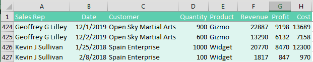
Start by making sure your data is sorted. The data below is sorted by customers in column C.
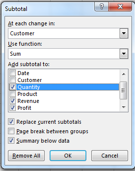
From the Data tab, choose Subtotals. The Subtotal dialog box always wants to subtotal by the leftmost column. Open the At Each Change In dropdown and choose Customer. Make sure the Use Function box is set to Sum. Choose all of the numeric fields, as shown here.
When you click OK, Excel inserts a subtotal below each group of customers. But, more importantly, it adds Group and Outline buttons to the left of column A.
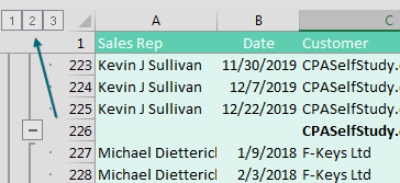
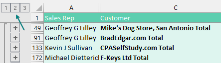
When you click the #2 Group and Outline button, the detail rows are hidden, and you are left with only the subtotal rows and the grand total. This is a beautiful summary of a detailed data set. Of course, at this point, the customers appear in alphabetic sequence. Derek from Springfield showed me that when the data is collapsed in the #2 view, you can sort by any column. In the figure below, a Revenue column cell is selected, and you are about to click the ZA sort button.
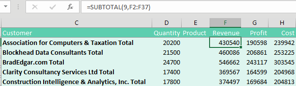
The top customer, Mike's Dog Store, comes to the top of the data set. But it does not come to row 2. Behind the hidden rows, Excel actually sorted a chunk of records. All of the Mike's detail rows moved along with the subtotal row.
If you go back to the #3 view, you will see the detail records that came along with the subtotal row. Excel did not rearrange the detail records; they remain in their original sequence.
To me, this is astounding on two fronts. First, I am amazed that Excel handles this correctly. Second, it is amazing that anyone would ever try this. Who would have thought that Excel would handle this correctly? Clearly, Derek from Springfield.
Bonus Tip: Fill in a Text Field on the Subtotal Rows
Say that each customer in a data set is assigned to a single sales rep. It would be great if you could bring the sales rep name down to the subtotal row. Here are the steps:
|
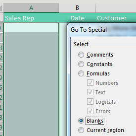
1. Collapse the data to the #2 view. 2. Select all of the sales rep cells, from the first subtotal row to the last customer subtotal row. Don't include the Grand Total row. At this point, you have both the visible and hidden rows selected. You need just the blank rows or just the visible rows. 3. At the right side of the Home tab, open the Find & Select dropdown. Choose Go To Special. In the Go To Special dialog, choose Blanks. Click OK. 4. At this point, you've selected only the blank sales rep cells on the Subtotal rows. In my case, the active cell is A49. You need a formula here to point one cell up. Type |
 |
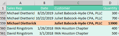
The results: The subtotal rows show the sales rep name in addition to the numeric totals.
Bonus Tip: An Easier Way to Fill in a Text Field on Subtotal Rows
Kimberly in Oklahoma City and Sarah in Omaha combined to provide a faster solution to getting the sales rep to appear on the Subtotal rows. Provided you only need the data in the #2 Summary View, this works amazingly well:
1. Click the #3 group and outline button to see all rows.
2. Select the first sales rep in A2.
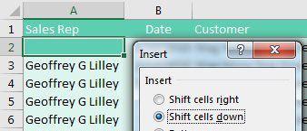
3. Press Ctrl++ and press Enter. In other words, while holding down Ctrl, press the + sign. This opens the Insert Cells dialog with "Shift Cells Down" selected. Pressing Enter is like pressing OK. This moves all of the sales reps down one row and leaves an ugly gap in A2 and the first row of every other customer.
But when you go back to the #2 view, the gaps disappear and the report is correct!
Bonus Tip: Format the Subtotal Rows
It is a little odd that Subtotals only bolds the customer column and not anything else in the subtotal row. Follow these steps to format the subtotal rows:
1. Collapse the data to the #2 view.
2. Select all data from the first subtotal to the grand totals.
3. Press Alt+; or select Home, Find & Select, Go To Special, Visible Cells Only.
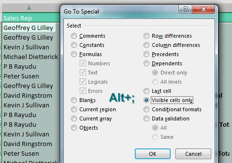
4. Click OK. Format the subtotal rows by applying bold and a fill color.
Now, when you go back to the #3 view, the subtotal rows will be easy to spot.
Bonus Tip: Copy the Subtotal Rows
Once you've collapsed the data down to the #2 view, you might want to copy the subtotals to a new worksheet. If so, select all the data. Press Alt+; to select only the visible cells. Press Ctrl+C to copy. Switch to a new workbook and press Ctrl+V to paste. The pasted subtotal formulas are converted to values.
Thanks to Patricia McCarthy for suggesting to select visible cells. Thanks to Derek Fraley for his suggestion from row 6.
This article is an excerpt from MrExcel 2024 Igniting Excel
Title photo by Markus Spiske on Unsplash